Lennard-Jones Potential

Equation

\[ V(r) = 4 \epsilon \biggl[ \biggl (\frac{\sigma}{r}\biggr)^{12} - \biggl (\frac{\sigma}{r}\biggr)^6 \biggr] \]

\[ \sigma = \frac{r_m}{2^{1/6}} \]

Here, epsilon is the energy minimum and r_m is the distance of the energy minimum.

Note the part of the equation inside the square brackets. Recall that negative energies represent a more favorable interaction. The attractive term (raised to the power of 6) is subtracted from the repulsive term (raised to the power of 12).

See the Lennard-Jones (L-J) potential on Wikipedia for more details. Also, L-J models are part of a wider set of models of Interatomic potentials.

Make plot of an example L-J potential

In the calculations and plot that follows, all distance units are in meters and energy units are in kJ/mol. I chose kJ/mol as the energy unit arbitrarily. I chose meters as the distance unit because the orders of magnitude at the atomic scale are the easiest to plot (note that the x-scale of the plot is marked in nanometers.)

Define constants

rmin and epsilon define shape of the potential and rmax is the maximum distance at which I calculate and plot the potential. My selection of values for rmin and epsilon are arbitrary and I selected them for ease of interpretation in the plot

import numpy as np
import matplotlib.pyplot as plt

rmin = 0.5e-9   # 2 angstroms
rmax = 1.0e-9  # 10 angstroms
epsilon = 1  # kJ/mol

Calculate and plot the potential

rs contains the radii that are in plot and vs contains the corresponding potentials. I calculate vs by NumPy array broadcasting which eliminates the need for a loop.

rs = np.linspace(rmin - 0.75e-10, rmax, 200)
sigma = rmin / 2**(1/6)
vs = 4 * epsilon * ((sigma/rs)**12 - (sigma/rs)**6)

fig, ax = plt.subplots(nrows=1, ncols=1, figsize=(10,7))
ax.set_xlim(min(rs), max(rs))
ax.set_ylim(min(vs)*1.1, max(vs))
ax.axhline(y=0, color='r', linestyle='dotted')
ax.plot(rs, vs)
ax.axvline(rs[vs.argmin()], color='orange')
ax.set_title(f'L-J Potential', size=20)
ax.set_xlabel('r (m)', size=15)
ax.set_ylabel('V (kJ/mol)', size=15)

Text(0, 0.5, 'V (kJ/mol)')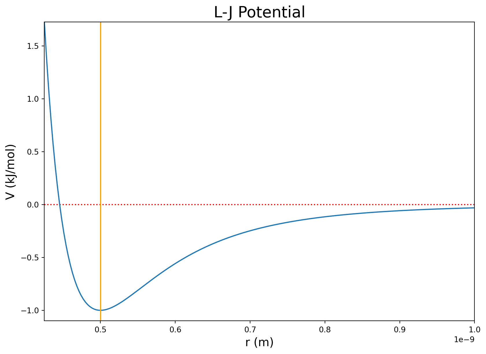

Discussion of the plot

I noted V(r) = 0 kJ/mol with a horizontal red dashed line and the position of the minimum potential with a vertical orange line.

Recall that the equation contains a repulsive term and an attractive term. The most favorable distance for this interaction is at 0.5 nm (5 angstroms) because that has the minimum energy. The repulsive term lies to the left of the orange line and rapidly increases as the radius approaches zero. This represents repulsion between atoms if they get too close. The attractive part of the potential lies to the right of the orange line and asymptotically approaches 0 as the atoms drift apart.