import matplotlib.pyplot as plt
import numpy as np
from scipy.integrate import quad
from math import pi, sqrt, exp, factorial


class QuantumHarmonicOscillator:
    """
    This models a harmonic oscillator. Parameters used throughout the methods
    are:

    v: The quantum of the harmonic oscillator
    k: The force constant
    mass_r: The reduced mass of the system. If you need to calculate this for a
            diatomic molecule, see the diatomic_reduced_mass() method below.

    The nomenclature of variable names follows Atkins and de Paula Physical
    Chemistry 8th ed, pp. 290-297.

    Atkins, P. W. & De Paula, J. Atkins’ Physical chemistry. (W.H. Freeman, 2006).
    """

    def __init__(self, mass_r, k):
        """
        Setup the values used by all methods in this model.

        Parameters
        ----------
        mass: float
            The reduced mass of the system, in kg

        k: float
            The force constant, in N/m
        """
        self.hbar = 1.054571817e-34
        self.k = k
        self.mass_r = mass_r
        self.omega = sqrt(k / mass_r)
        self.max_nu = 6

    @staticmethod
    def diatomic_reduced_mass(mass_1, mass_2):
        """
        Computes the reduced mass of a diatomic system. In order to provide
        meaningful results, please use the exact isotopic mass for your molecule.

        Parameters
        ----------
        mass_1: float
            The mass of the first atom in kg.

        mass_2: float
            The mass of the second atom in kg.
        """
        return mass_1*mass_2/(mass_1+mass_2)

    def hermite(self, v, gamma):
        """
        Returns the value of the v-th (nth) Hermite polynomial evaluated on gamma

        The v and gamma notation follows Atkins' Physical Chemistry 8th ed.

        Parameters
        ----------
        v: int
            The v-th (nth) Hermite polynomial

        gamma: float
            The value to calculate with the Hermite polynomial

        Returns
        -------
        float
            The value of the v-th Hermite polynomial evaluated with gamma.

        Raises
        ------
        Exception
            Raises an exception if the nth Hermite polynomial is not
            supported.
        """
        if v == 0:
            return 1
        elif v == 1:
            return 2 * gamma
        elif v == 2:
            return 4 * gamma**2 - 2
        elif v == 3:
            return 8 * gamma**3 - 12 * gamma
        elif v == 4:
            return 16 * gamma**4 - 48 * gamma**2 + 12
        elif v == 5:
            return 32 * gamma**5 - 160 * gamma**3 + 120 * gamma
        elif v == 6:
            return 64 * gamma**6 - 480 * gamma**4 + 720 * gamma**2 - 120
        else:
            raise Exception(f"Hermite polynomial {v} is not supported")

    def max_v(self):
        """
        Returns
        -------
        int
            The maximum v value for the instance.
        """
        return 6

    def energy(self, v):
        """
        Calculate the energy at the given level v of the system

        Parameters
        ----------
        v: int
            The quantum vmber v for the energy level of this system

        Returns
        -------
        float
            Energy of the system in Joules.
        """
        return (v + 0.5) * self.hbar * self.omega

    def energy_separation(self):
        """
        Returns
        -------
        float
            The energy difference between adjacent energy levels in Joules.
        """
        return self.hbar * self.omega

    def wavefunction(self, v, x):
        """
        Returns the value of the wavefunction at energy level v
        at coordinate x.

        Parameters
        ----------
        v: float
            Energy level of the system.

        x: float
            x coordinate of the particle in m.

        Returns
        -------
        float
            Value of the wavefunction v at x.
        """
        alpha = (self.hbar**2 / self.mass_r / self.k) ** 0.25
        gamma = x / alpha
        normalization = sqrt(1 / (alpha * sqrt(pi) * 2**v * factorial(v)))
        gaussian = exp((-(gamma**2)) / 2)
        hermite = self.hermite(v, gamma)
        return normalization * hermite * gaussian

    def wavefunction_across_range(self, v, x_min, x_max, points=100):
        """
        Calculates the wavefunction across a range.

        Parameters
        ----------
        v: int
            The quantum vmber of the system.

        x_min: float
            The minimum x value to calculate.

        x_max: float
            The maximum x value to calculate.

        points: int
            The vmber of points across the range

        Returns
        -------
        np.array, list
            The first array are the x coordinates, the second list are the
            float values of the wavefunction.
        """
        xs = np.linspace(x_min, x_max, points)
        ys = [self.wavefunction(v, x) for x in xs]
        return xs, ys

    def prob_density(self, v, x_min, x_max, points=100):
        """
        Returns the probability density between x_min and x_max for a given
        vmber of points at energy level v.

        Parameters
        ----------
        v: int
            Quantum vmber of the system.

        x_min: float
            Minimum of length being calculated. Probably negative. Units are
            meters.

        x_max: float
            Maximum of length being calculated. Probably positive. Units are
            meters.

        points: int
            The vmber of points to compute the probability density for

        Returns
        -------
        np.array, list
            The first array is the list of x coordinates. The list are the
            corresponding values of the probability density.
        """
        xs = np.linspace(x_min, x_max, points)
        ys = [self.wavefunction(v, x) ** 2 for x in xs]
        return xs, ys

    def integrate_prob_density_between_limits(self, v, x_min, x_max):
        """
        As a way of testing the methods in this class, provide a way to
        integrate across the wavefunction squared between limits.

        Parameters
        ----------
        v: int
            Quantum vmber of the system.

        x_min: float
            lower bound of integration

        x_max: float
            upper bound of integration
        """

        def integrand(x):
            return self.wavefunction(v, x) ** 2

        result, _ = quad(integrand, x_min, x_max)
return resultIntroduction
In this post, I will define Python code that models the quantum harmonic oscillator. This page follows page 290 to 297 in Physical Chemistry, 8th Ed. by Peter Atkins and Julio de Paula for the math to create and examples to test the code in this post.
The following equations describe its energy levels:
\[ \omega = \sqrt{\frac{k}{m}} \]
\[ E_{\nu} = \Bigl(\nu + \frac{1}{2}\Bigr) \hbar \omega \]
\[ \nu = 0, 1, 2, \dots \]
The following equations describe its wavefunction:
\[ \alpha = \Biggl(\frac{\hbar^2}{mk}\Biggr)^{1/4} \]
\[ \gamma = \frac{x}{\alpha} \]
\[ \psi_{\nu}(x) = N_{\nu} H_{\nu}(\gamma) e^{-\gamma^{2}/2} \]
where \(H\) is a Hermite polynomial. The form of the first six Hermite polynomials are on page 293 of the text and are also implemented in the QuantumHarmonicOscillator class shown in the Python source code section below. Here is a sampling of the first three:
\[ H_0(\gamma) = 1 \]
\[ H_1(\gamma) = 2 \gamma \]
\[ H_2(\gamma) = 4 \gamma^2 - 2 \]
Example 9.3 on page 294 demonstrates the derivation of the normalization constant \(N_{}\), which results in the following expression for the normalization constant:
\[ N_{\nu} = \sqrt{\frac{1}{\alpha \pi^{1/2} 2^{\nu} \nu!}} \]
The Python class for the harmonic oscillator
Test the class with 1H35Cl Properties
The 1H35Cl molecule has a bond with the following physical properties (the mass is of the proton in Hydrogen).
\[ k = 516.3 N/m \]
\[ m = 1.7 \times 10^{-27} kg \]
k = 516.3
mass = 1.7e-27
x_min = -0.5e-10
x_max = 0.5e-10
points = 1000
qho = QuantumHarmonicOscillator(k=k, mass_r=mass)
nus = range(qho.max_nu + 1)
fig, axs = plt.subplots(nrows=len(nus), ncols=2, figsize=(10, len(nus) * 5), sharex=True)
for idx, nu in enumerate(nus):
    xs_wavefunction, ys_wavefunction = qho.wavefunction_across_range(nu, x_min, x_max, points)
    xs_prob_density, ys_prob_density = qho.prob_density(nu, x_min, x_max, points)
    integrated = qho.integrate_prob_density_between_limits(nu, x_min, x_max)
    axs[nu, 0].set_title(f'ν={nu}', size=15, color='r')
    axs[nu, 0].set_ylabel(f'Ψ{nu}(x)', size=15, color='b')
    axs[nu, 0].set_xlabel('x', size=15)
    axs[nu, 0].set_xlim(x_min, x_max)
    axs[nu, 1].set_title(f'ν={nu}, ∫Ψ{nu}^2={round(integrated)}', size=15, color='r')
    axs[nu, 1].set_ylabel(f'Ψ{nu}(x)^2', size=15, color='b')
    axs[nu, 1].set_xlabel('x', size=15)
    axs[nu, 1].set_xlim(x_min, x_max)
    axs[nu, 0].plot(xs_wavefunction, ys_wavefunction)
    axs[nu, 1].plot(xs_prob_density, ys_prob_density, color='g')

plt.show()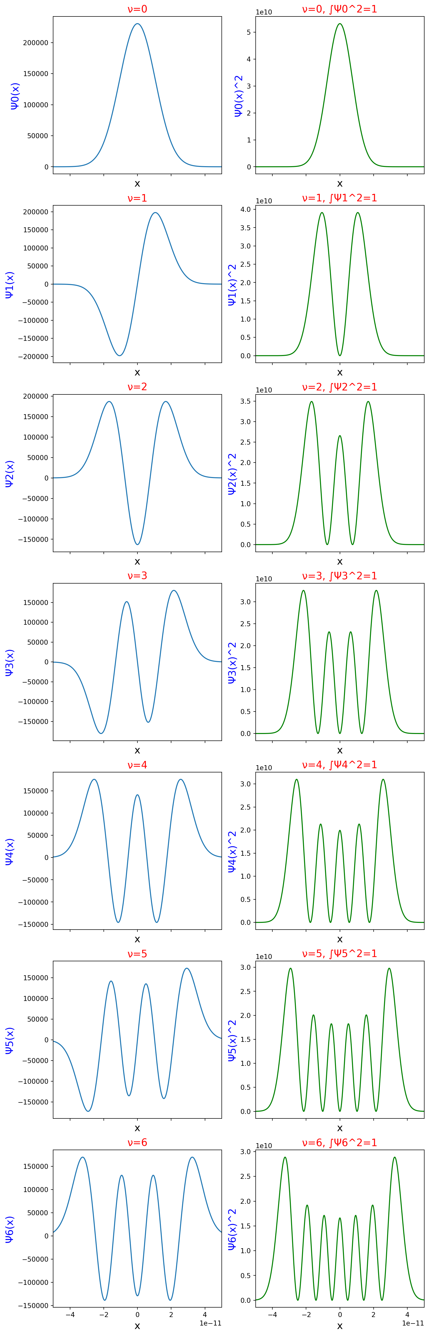
In the plots of Figure 1, there are two columns. The left column is a plot of wavefunctions at different nu levels, each with a title indicating the level of the plot. The right column has plots of the squares of the wavefunctions. Like the left column plots, the titles of these plots contain the nu value that created them. In addition, the titles include an integral in their titles. These integrals all have a value of one, meaning each square of the wavefunction displays the probability throughout the entire space of wavefunction.
Testing the energy level calculation from Illustration 9.3
Using the 1H35Cl specifications from above, I will calculate the zero point energy and energy separation following Atkins and de Paula, Illustration 9.3. The 1H35Cl specifications are:
\[ k = 516.3 N/m \]
\[ m = 1.7 \times 10^{-27} kg \]
However, the book uses k=500 N/m and I will make that assumption to maintain consistency.
k = 500
mass = 1.7e-27
mol = 6.022e23
qho = QuantumHarmonicOscillator(k=k, mass_r=mass)
energy_sep_kj_mol = qho.energy_separation() * mol / 1000  # Convert to kJ/mol
print(f'energy sepration between ν and ν+1, {energy_sep_kj_mol} kJ/mol')
zero_point_kj_mol = qho.energy(v=0) * mol / 1000
print(f'zero-point energy {zero_point_kj_mol} kJ/mol')
first_excitation_thz = (qho.energy(v=1) - qho.energy(v=0)) / 6.626e-34 / 1e12
print(f'First excitation energy {first_excitation_thz} THz')
energy sepration between ν and ν+1, 34.44113487055476 kJ/mol
zero-point energy 17.22056743527738 kJ/mol
First excitation energy 86.31480043180733 THzFrom the answers given in the book, this gives my model the following differences.
delta_energy_sep = (round(energy_sep_kj_mol) / 34.0 - 1) * 100
print(f'delta energy separation {delta_energy_sep}%')
delta_zero_point = (round(zero_point_kj_mol) / 15.0 - 1) * 100
print(f'delta zero point energy {delta_zero_point}%')
delta_first_excitation = (round(first_excitation_thz) / 86.0 - 1) * 100
print(f'delta first excitation {delta_first_excitation}%')
delta energy separation 0.0%
delta zero point energy 13.33333333333333%
delta first excitation 0.0%